Setup
git clone https://github.com/mehradans92/Gelator-Transparency-Predictor.git
cd /home/mehrad/Gelator-Transparency-Predictor
uv venv latent-space
source latent-space/bin/activate
uv pip install -r requirements.txtIntroduction
Traditionally, theory and algorithms of various machine learning methods have been mostly developed for problems with linear settings [1]. These linear methods such as multiple linear regression (MLR) [2], ridge regression (RR) [3], principle component regression (PCR) [4] and partial least squares regression (PLSR) [5] have become widely popular in chemistry for predicting the properties of new samples [6]. In practice, however, these methods may be inapplicable to complex real-world chemical systems, where the relationship between the process variables are nonlinear [7]. For instance, according to Bernoulli's equation, the pressure drop and flow rate have a squared relationship or the outlet temperature and the concentration of species in a chemical reactor are nonlinearly related, given complex reaction kinetics and energy balance.
Kernel methods [8–12] solve the nonlinearity problem by using a simple linear transformation manner. The key idea is to project the data onto a higher-dimensional space, where linear methods are more applicable [13] and chances of over-fitting are less likely [14]. The kernel methods are performed in two successive steps: First, the training data in the input space are nonlinearly mapped onto a much higher dimensional feature space, where sometimes even unknown features are induced by the kernel [15]. In the second step, a linear method is applied to find a linear relationship in that feature space in a regression or a classification setting. Since everything is formulated in terms of kernel-evaluations, there is no need for performing any explicit calculations in the high-dimensional feature space [16]. This allows an efficient solution to the highly nonlinear convex optimization problems encountered in chemistry [17–22].
In this work, we focus on applying kernel ridge regression (KRR) to infer the observable in terms of a linear expansion of the gelation experimental space and perform a binary classification for the transparency of anionic gelators. The low number of experimental data points, paired with a highly non-linear learning problem makes kernel learning a suitable choice to our setting.
Theory
Kernel Methods
With a kernel, data can be nonlinearly mapped from original input space \(\mathcal{R}^{D}\) onto a feature space \(\mathcal{R}^{F}\), with input and feature dimension \(D\) and \(F\), respectively.
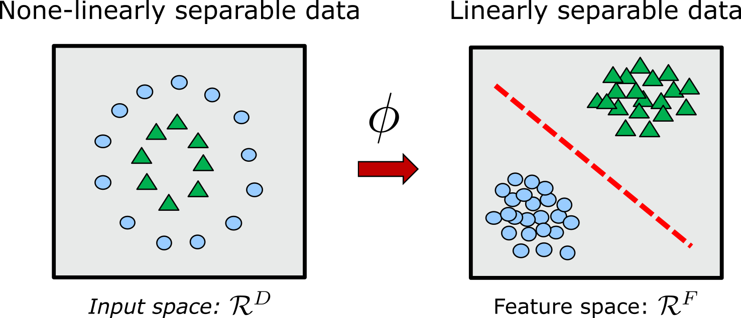
For transformation (mapping) \(\phi:\mathcal{R}^{D} \rightarrow \mathcal{R}^{F}\), a kernel function is defined as
\[K(\mathbf{x},\mathbf{y}) = \langle \phi(\mathbf{x}), \phi(\mathbf{y})\rangle_F\]A key requirement is that \(\langle\cdot\rangle_F\) is a proper inner product. This means that a kernel is required to work on scalar products of type \(\mathbf{x}^T\mathbf{y}\) that can be translated into scalar products \(\phi(\mathbf{x})^T\phi(\mathbf{y})\) in the feature space. On the other hand, as long as \(F\) is an inner product space, the explicit representation of \(\phi\) is not necessary and the kernel function can be evaluated as [23]:
\[K(\mathbf{x},\mathbf{y}) = \phi(\mathbf{x})^T\phi(\mathbf{y})\]This is also known as the kernel trick [11], and interestingly, many algorithms for regression and classification can be reformulated in terms of the kernelized dual representation, where the kernel function arises naturally [10]. Using the kernel trick, we never have to explicitly do the computationally expensive transformation \(\phi\).
A key concept here is that the transformation can be done implicitly by the choice of the kernel. In specific, the kernel encodes a real valued similarity between inputs \(\mathbf{x}\) and \(\mathbf{y}\). The similarity measure is defined by the representation of the system which is then used in combination with linear or non-linear kernel functions such as Gaussian, Laplace, polynomial and sigmoid kernels. Alternatively, the similarity measure can be encoded directly into the kernel, leading to a wide variety of kernels in the chemical domain [24]. In this setting, the defined binary kernel function needs to be non-negative, symmetric and point-separating (i.e. \(\langle x,x' \rangle = 0\) if and if only \(x=x'\)) [25]. For a given numerical feature we can use distance or \(l_2\) norm (Euclidean distance), whereas for a categorical feature, hamming distance is applicable.
Kernel Ridge Regression
Consider a data set containing \(N\) input samples \(\{x_i\}_{i=1}^N\), labeled as \(\{y_i\}_{i=1}^N\). In ridge regression, loss function
\[L(w) = \frac{1}{N}\sum_{i=1}^{N} (y_i - \vec{w}^T \vec{x_i})^2 + \lambda \cdot \|w\|^2\]is minimized with respect to weight coefficients \(w\), where hyperparameter \(\lambda\) is used for regularization, which penalizes the norm of the weights. Increasing \(\lambda\) results in smoother functions that avoid the pure interpolation of the training data and thus, reduces overfitting. Despite having a good stability in terms of the generalization error, linear ridge regression needs a non-linear variant to better capture the features of complex non-linear systems.
This non-linear variant is obtained by kernelizing the ridge regression formulation. The dual form of kernel ridge regression (KRR) is given by
\[\hat{y} = \sum_{i=1}^N \alpha_i \cdot \langle \vec{x},\vec{x_i} \rangle\]where \(\hat{y}\) is a model's prediction for unknown new data sample \(x\), given known training data \(x_i\). \(\alpha\) is obtained from
\[\alpha=(\lambda\cdot \mathbf{I} + \mathbf{K})^{-1}y\]where \(\mathbf{I}\) is the identity matrix and \(\mathbf{K} \in \mathcal{R}^{N\times N}\) is the Gram matrix, defined as \(\mathbf{K_{ij}}=k(x_i,x_j)\).
Methods
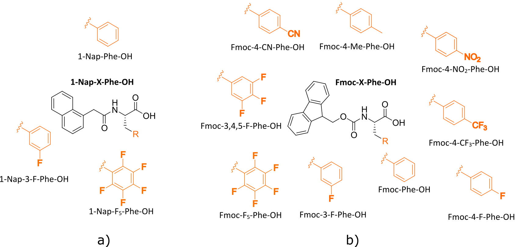
Before defining this representation, we provide a brief description of the classification problem. The gelation experiment dataset contains features that include different experimental conditions such as the chemical structure, gelator concentration and equivalents of Glucono Delta Lactone (GdL) added during the experiment. The latter is added to the solution to trigger gelation process. This dataset for training is obtained by creating 29 anionic gelators under various alterations of the three mentioned features. The resulting gelators are either transparent or opaque, making this a binary classification problem.
Representation of the System
A key ingredient in kernel-based methods is the representation of the physical system. In the gelation experiment, the chemical structures vary given different functional groups at their \(N\) terminus.
The similarity between two chemical structures \(A\) and \(B\) is measured by their hamming distances defined as
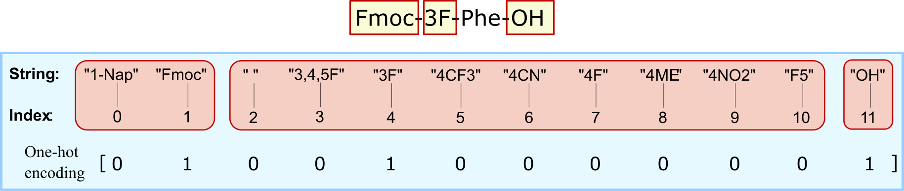
\[\delta_{\text{hamming}} = L - \sum(\text{ohe}(A)\cdot \text{ohe}(B))\]where \(\text{ohe}\) is the one-hot encoding for the chemical structure and \(L\) is the total length of positions. Hamming distance between two strings (of equal length), is the number of the positions at which the corresponding symbols are different. In other words, it measures the number of minimum substitutions required to change one string to another.
The one-hot-encoding is a trick of encoding categorical variables such as a set of strings into numerical values as "0"s and "1"s. We can consider having three labels in the strings, each representing different parts of a chemical structure name. Each label can be substituted by limited set of strings that represent the functional group. In this setting, we are doing a multi-class classification problem for each label. This means that there can be only a single "1" in the positions of the corresponding functional group for each label, with the rest of the values set to "0". Given this definition and the formulation of hamming distance, the maximum distance between two chemical structures is three, meaning that all three positional strings are not similar.
The other features include gelator concentration and equivalents of GdL, which are both a scalar. We define distance \(d\) as the absolute numerical difference, to ensure a positive kernel for each of those features. With this definition we can calculate the overall distance \(D\) between the datapoints in each experiment given by
\[D(A,B) = \sqrt{\delta_{\text{hamming}}^2(A,B) + d_{\text{conc}}^2(A,B) + d_{\text{GdL}}^2(A,B)}\]Note that all the features are normalized before distance calculations. The binary labels are defined based on the experiment outcome for gelator's transparency, i.e. "0" for opaque and "1" for transparent.
Results
The model is trained in 29 gelation experiment data using KRR with kernels described above. The predicted labels from KRR are numerical float values between zero and one are decoded into the discrete representation of the true labels. By considering a middle threshold of 0.5, predictions beyond 0.5 are classified are transparent and opaque otherwise. This definition allows us to consider an uncertainty in predictions by finding the Euclidean distance between the new experiment data and all the training set.
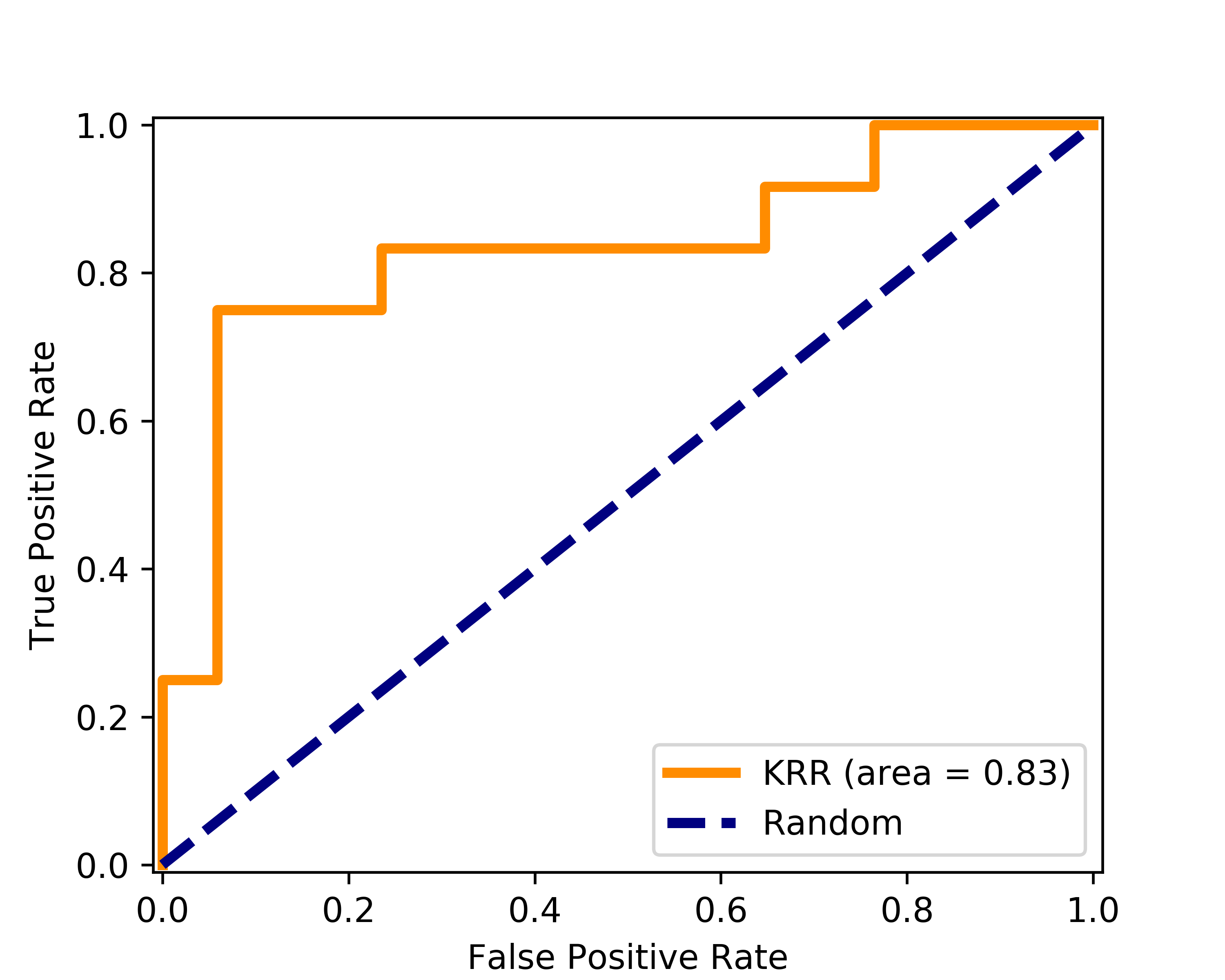
Classifier's generalization error was minimized with \(\lambda\) of 1 after performing leave-one-out cross-validation (LOOCV). This error was found to be 0.83, which demonstrates on the applicability of KRR method for small datasets. The accuracy of the model is evaluated with the receiver operating characteristic curve (ROC) with area-under-curve (AUC) of 0.83.
Discussion
In this work, we demonstrated on applying kernel ridge to regression to embed the small gelation experimental data into a higher dimensional feature space and discover a calibrated linear relationship, while avoiding overfitting. In this setting, kernel learning was advantageous in two ways. First, it helped by solving a non-linear problem, where linear methods would have failed. Secondly, using kernel learning allowed us to expand the number of weights from number of features to number of training datapoints.
Proper description of the physical system is a key ingredient to kernel methods. In fact, this representation defines the function class from which the model is chosen and how it performs. Ideally speaking, this representation of data should distill relevant information about the learning problem in a concise manner, such that learning is possible even for small number of examples. In this regard, finding an appropriate representation of data can become a central problem. In contrast, deep neural networks can learn this representation from the data in a layer-wise fashion [26, 27]. Considering these observations, it will be of interest to apply this problem to different representation of the chemical structure such as self-referencing embedded strings (SELFIES) [28] or simplified molecular-input line-entry system (SMILES) [29] that allows to incorporate some chemical intuition into the model.